Indexology^® Blog

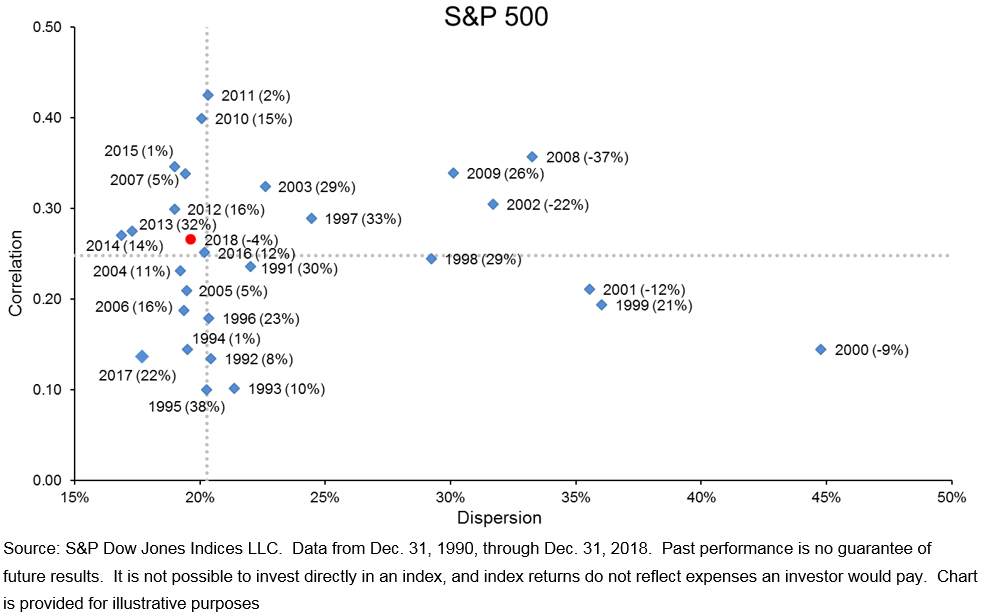
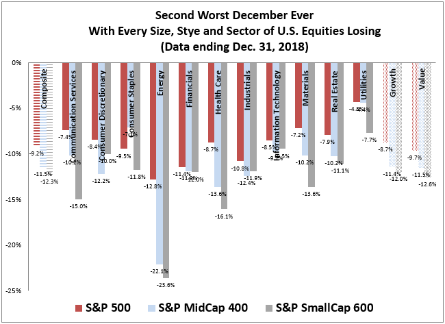
As the ball dropped this New Year’s Eve, most investors were more than happy to bid adieu to what proved to be a volatile end to 2018. The fourth quarter began with the October sell-off, which was just the start of a highly volatile quarter. The S&P 500^® fell almost 7% in October alone, with losses accelerating into the end of the year during what is likely to be one of the worst Decembers on record.

Large equity market drawdowns such as these remind us of the importance of portfolio diversification. Traditionally, this has been achieved by building multi-asset portfolios that combine complementary asset classes such as stocks and bonds.

First generation multi-asset strategies, exemplified by a 60/40 allocation, seek to create balanced portfolios by diversifying across asset classes in fixed proportions. However, this technique does not maximize diversification benefits because it ignores the risk contribution of each asset class.

The recognition of these shortcomings led to the development of a class of investment strategies called risk parity, which seeks to equalize the risk contribution of each asset class. The primary goals of risk parity are to provide a smoother return profile and minimize losses from equity market drawdowns like we saw in the fourth quarter of 2018—so let’s examine how they performed.

While each of these portfolios also posted negative returns, the losses seen in the 60/40 portfolio and the S&P Risk Parity Indices were modest compared with the large drawdowns witnessed in equity markets (see Exhibits 1 and 2). As one might expect, the “risk-balanced” S&P Risk Parity Indices outperformed the global 60/40 portfolio across each volatility target.

Now let’s take this analysis to the next level and examine the asset class performance attribution within these indices (using excess returns). The S&P Risk Parity Indices comprise three asset class sub-components: equities (broad indices across the U.S., Europe, and Asia), fixed income (sovereign bonds across the U.S., Europe, and Asia), and commodities (energy, softs and livestock, grains, and metal sub-sectors).

The equity component drove the bulk of the negative performance, contributing a loss of 4.72%. The fixed income component offset some of the negative equity performance, contributing a gain of 2.79%, with the majority of the positive performance coming in December. The commodities component did not fare as well, contributing a loss of 2.97%, which in essence canceled out the diversification benefit provided by fixed income.

Q4 2018 may not be a stellar example of the power of diversification, but it underlines the need to maximize the so-called “only free lunch in finance.” When equities are given an outsized risk allocation, equity market losses like those seen in Q4 2018 will dominate portfolio performance. However, when each asset class is given equal footing, the diversification benefits have a better chance of shining through. Given the opportunity, investment strategies such as the S&P Risk Parity Indices have the potential to help smooth out drawdowns and improve risk-adjusted returns.

In a prior blog, Getting to Know the S&P/BMV IPC – An Iconic Representation of the Mexican Equity Market, we examined the evolution of the S&P/BMV IPC and tracked its role from being a financial market indicator to serving as the basis for index-linked liquid investment products. In this blog post, we look at the investability criteria incorporated in the index methodology, allowing it to meet the liquidity needs of market participants and index-linked investment products.

The investability of an index is a function of two variables—the liquidity of the underlying constituents and the weight of the securities in the index. For instance, a security with low liquidity should not necessarily have a high weight in the index, all else being equal. Moreover, the investability of an index determines its investment capacity.

Therefore, index design should strive to achieve an investable and replicable index for the target market. With that in mind, we look at the index mechanics of the S&P/BMV IPC and review how the methodology addresses liquidity needs. Some of the most relevant points were:

• Weighting scheme: In 1999,[1] the S&P/BMV IPC methodology changed from total market-cap weighted to a float-adjusted market-cap weighting scheme. The index also employs additional constraints to reduce concentration risk: no single stock’s weight can exceed 25% and the aggregate weight of the five largest stocks cannot exceed 60%.
• Minimum float inclusion criteria: The free float factor measures the percentage of company shares available to be traded in a market. The S&P/BMV IPC methodology added this requirement in 2012[2] as inclusion criteria for constituents. To be part of the S&P/BMV IPC, stocks must have an investable weight factor (IWF) of at least 10%.
• Volume-weighted average price (VWAP) float-adjusted market cap inclusion criteria: To be part of the S&P/BMV IPC, stocks must have a minimum VWAP float-adjusted market cap of MXN 10 billion (MXN 8 billion for current constituents). VWAP float-adjusted market cap is calculated by multiplying the number of shares outstanding by the assigned company’s IWF and by the VWAP over the prior three-month period.
• Median daily value traded (MDVT) inclusion criteria: to be part of the S&P/BMV IPC, stocks must have a MDVT of at least MXN 50 million (MXN 30 million for current constituents) over the prior three- and six-month periods.
• Median traded value ratio (MTVR) inclusion criteria: Stocks must have an annualized MTVR of at least 25% over the prior three- and six-month periods.

Do these index mechanics improve the overall liquidity profile of the index? We reviewed the daily trading volume of the S&P/BMV IPC constituents to find out. As of Nov. 30, 2018, the six-month MDVT of the index was around USD 8.80 million on average, compared with that of S&P/BMV IPC CompMx constituents at USD 5.29 million. Hence, the S&P/BMV IPC was nearly 50% more liquid than the broader index.

A quick capacity analysis using the index composition as of Nov. 30, 2018, and the constituents’ six-month MDVT showed that a portfolio of USD 140 million could be completely traded in a single day (assuming 100% of the six-month MDVT). On the other hand, trading the same portfolio size on the broader S&P/BMV IPC CompMx would take double that amount of time.

Currently, the S&P/BMV IPC serves as the underlying benchmark for an ETF with assets of over USD 3 billion.[3] The size of this index-linked product is a testament to the importance of having a liquid and investable underlying benchmark.

[1]   The S&P/BMV IPC Turns 40

[2]   The S&P/BMV IPC Turns 40

[3]   Source: ETFGI. https://etfgi.com/news/press-releases/2018/10/etfgi-reports-assets-etfs-and-etps-listed-latin-america-see-net-inflows. ETFGI is the leading independent research and consultancy firm on trends in the global ETF/ETP ecosystem and is based in London, England. Deborah Fuhr, Managing Partner, co-founder, ETFGI website www.etfgi.com.

Equities have historically offered promising growth potential, but we have seen time and again how suddenly and severely the equity markets can be affected by events that are difficult to predict, and 2019 is not likely to be an exception. Losses can have a greater impact on portfolios than gains because the money remaining after the loss must work hard to recover just to break even.

Losses can happen more often than expected…

S&P 500 INDEX DRAWDOWNS[1]

…and it can take years to recover

YEARS TO RECOVER WITH ANNUAL RATE OF 5%[2]

Traditionally, investors have relied on diversifying equities with bonds, or market timing, to help minimize their risks from losses. But these strategies may be challenged in certain market environments.

60/40 may not be the answer

Many investors maintain a typical 40% allocation to fixed income investments to provide a counterbalance to equities during times of market volatility. However, bonds may decline at the same time as equities, as happened in October 2018, negating the expected counterbalance benefit. Fixed income may also be challenged when interest rates rise and lose purchasing power in an inflationary environment.

Being cautious does not mean being in cash

Investors who sell at the first sign of market downturns and wait on the sidelines in cash for the market to recover can miss out on top-performing days, which can have a big impact on returns. Further, like fixed coupon bonds, cash loses purchasing power in an inflationary environment.

A defensive options strategy can provide protection plus potential growth

An alternative approach that may help protect an investment involves the use of options—instruments that seek to provide a contractual level of certainty that other approaches lack.

A defensive “buffer protection” strategy, utilizing a combination of call and put options overlaid on an exposure to a given index, offers an alternative risk management solution. This type of strategy provides a “buffer” of protection against the first 10% of losses in the chosen index while capturing potential growth to a maximum capped gain (“cap”) over a period of approximately one year.

The cap level is set at the start of the period, such that the 10% downside protection is paid for by giving up potential returns above the cap. The returns of the strategy will be a function of the level of the index at the end of the period relative to its level at the start of the period.

Defensive buffer protection option strategies are typically implemented in structured notes and annuities with a single strategy of one-year maturity. However, the single strategy, one-year maturity creates acute timing risks, locking investors into one specific cap and buffer for an entire year. This prevents investors from capitalizing on new buffer levels or upside caps over the course of the year as the chosen index moves up or down.

The timing risks associated with a single strategy, one-year maturity can be mitigated through the same “laddering” technique used by bond investors. Equity investors seeking persistent defensive protection can build a laddered portfolio of defensive options strategies with maturities ranging from one to 12 months. In this manner, each month a defensive options strategy would mature and be rolled forward for another 12 months. This allows the downside protection and cap levels to reset and stay current to the prevailing market conditions for a portion of the investment, which can be an advantage in a rising or falling market environment.

The Cboe S&P 500 Buffer Protect Index (ticker: SPRO) employs such a strategy, using a laddered portfolio of 12 Buffer Protect Strategies designed to protect the first 10% of losses in the S&P 500 while capturing growth to a maximum capped gain.

[1] Calculated using Bloomberg data as the percentage negative return on a date from the highest level by the S&P Index prior to that date.

[2] Calculated using the formula TimeToRecovery = -Ln(1-OneTimeLoss)/Ln(1+RecoveryRate).

In 2018, the S&P 500 declined for the first time in 10 years. The year’s 4% decline is obviously de minimis compared to 2008’s 37% plunge, though investors may feel it more keenly since the fourth quarter’s 14% decline erased what had been a profitable year.  Nonetheless, the risk landscape changed dramatically in 2018 compared to the lethargy of 2017.

We find it helpful to view market volatility through the lens of dispersion and correlation.  The graph below compares annual average dispersion and correlation levels for the past 28 years.  Between 1991 and 2017, there had been only four years in which the index was down; all coincided with very high dispersion.  2018’s relatively modest decline occurred in a different environment – average dispersion for the year ran slightly below its historical median.  The data suggest that while very high dispersion doesn’t guarantee a large decline, large declines have not occurred in the absence of very high dispersion.

DISPERSION-CORRELATION MAPS (RETURNS)

In December 2018 alone, the S&P 500 declined 9%, so it’s appropriate to observe that month’s data relative to other periods of market weakness.  The dispersion-correlation map below juxtaposes December 2018 against monthly levels in 2001 and 2008.  Even in December, dispersion lay below its historical median; the month’s surge in volatility was driven by a surge in correlation.  Dispersion would have to rise dramatically to approach the levels we saw in the last two market crashes.

The S&P 500 lost 9.2% in its second worst December on record – only behind December 1931 when the index lost 14.5%.  However, the widespread losses across sectors, styles and sizes in the broad U.S. equity market was remarkable with every major segment down in December.  Only 9 times in history has every segment of the U.S. equity market lost in a month (with all sector data starting in 1995 and style data in 1997.)   Those months were Aug. 2015, Sep. 2011, May and Jun. 2010, Jan. and Feb. 2009, Oct. 2008, and Jul. and Sep, 2002.

Not only was every segment of U.S. equities negative in December but 33 of 42 segments had their worst December ever,  For the 9 other segments, 7 recorded their 2nd worst Decembers and 2 had their 3rd worst Decembers.  Despite the December records, none of the 42 segments of the market posted their worst month ever, but the S&P MidCap 400  lost 11.5%, recording its 4th worst month ever, with the S&P 400 Health Care down 13.6%, S&P 500 Energy -12.8%, S&P 600 Consumer Staples -11.8% and S&P 600 Energy -23.6%, all recording their 3rd worst months ever.

As bad as December was, it was only partly responsible for the drawdowns experienced this year.  In fact, in most segments, December’s loss didn’t even account for half the total bloodshed.  Only 12 of 42 segments lost more than half their total drawdown in December: S&P 600 Utilities 63%, S&P 500 Real Estate 62%, S&P 400 Communication Services  62%, S&P 400 Real Estate  57%, S&P 600 Real Estate  57%, S&P 500 Health Care 56%, S&P 600 Communication Services 55%, S&P 600 Consumer Staples 55%, S&P 500 Consumer Staples 55%, S&P 400 Health Care 53%, S&P 600 Health Care 53%, and S&P 600 Financials 52%.  

Although health care and utilities declined in December for more than half their total drawdowns, they still held up relatively well for the year.  Overall, health care was the only sector with big enough early gains, especially in small caps to survive the year in positive territory.  The small caps outperforming large caps in health care can be due to deal making, increased expectations for acquisition of smaller companies, stronger innovation from smaller companies and that smaller companies may be more immune to concerns of regulatory pressures in healthcare.

That said, the S&P SmallCap 600 Health Care index still posted its worst quarter ever, losing 23.1%, due to the slowing growth of health care spending.  The S&P SmallCap 600 Industrials also logged its worst quarter ever, losing 23.5%, mainly due to a slowing economy and trade tensions.  While the S&P 500 Energy had its worst 4th quarter, losing 24.4%, it was not enough to push it into its worst year, but still only lost about half of the smaller companies in the sector.  If oil prices rise, and inflation picks up, small caps may get the benefit of the uptick since they are less hedged than the bigger energy companies.

What’s next for equities is impossible to know for sure, especially when there has only once been a December this bad.  While the year ended down 6.2% for the S&P 500, its worst in a decade, there were 22 years prior with worse returns.  In the Januaries following those 22 years, only 7 were negative, and the average return was 7.1%.  In the 22 years following the years worse than 2018, 9 were negative with an average of 1.0%, and of the 7 negative Januaries, 4 of those years ended negative in 1932, 1941, 1974 and 2002.  On average in all Januaries, small caps have lost 48 basis points while large caps gain 8 basis points and mid caps win gaining 39 basis points, and historically continue to win through the first quarter.

Though the market is hard to time, positioning for the rebound matters, especially by size and sector.  Mid-caps may do well in these first bull-market days since they are generally not as risky as smaller companies, yet have solid infrastructure but are nimble enough to take advantage of opportunities, especially overseas if the dollar drops.  Regardless of size, the financial and real estate sectors have done best on average in the first days of a new bull. Every size of these sectors develop into a bull market in the first 20 days on average after S&P 500 bottoms with large- and mid-cap financials returning nearly 28%. Even in just the first 3 days, the average returns of these segments were between 11.3% and 15.4%.

Is this time the same or different? Most of the time the markets come in cycles but there are some current issues to be focusing on now.  Despite decent consumer spending and manageable debt levels, low unemployment and wage growth and a growing economy – even if slowing, there are broader systematic risks impacting the world like slowing Chinese and European growth, trade tensions, Brexit, slowing housing and rising interest rates,