Indexology^® Blog

Although the low volatility anomaly was first documented more than 40 years ago, it was the trepidation and volatility in the years following the most recent financial crisis that propelled the concept to the forefront of investor interest.  In recent years, the phenomenon has been well covered, by both academics and the investment community, in the form of innovative financial instruments that exploit the anomaly and subsequent attraction of assets to those vehicles.  The low volatility anomaly exists not just in the U.S., but instead seems to be universal.  The current debate is less focused on the existence of a low volatility effect and more on the construction of various strategies to exploit the phenomenon.

In the U.S., for example, the S&P 500^® Low Volatility Index outperformed its benchmark, the S&P 500, from 1991 to 2014 by 101 bps compounded annually—with 31% less volatility.  What is the reason for its success?  Our rankings-based method of portfolio construction not only screens for stocks by factor, it also weights by factor (or the inverse of the factor, in this case) to achieve its objective.  This methodology has resulted in large sector weights, historically.

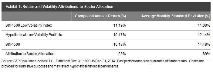
However, strategic sector tilts don’t paint the complete picture here.  If we only apply the returns of the S&P 500 sectors to the respective sector weights in S&P 500 Low Volatility Index over the last 24 years, the “hypothetical” low volatility portfolio can account for 69% of the total risk reduction.  This means that being in the “correct” sector during this period accounted for more than two-thirds of the volatility reduction achieved by the S&P 500 Low Volatility Index (see Exhibit 1).  In the same period, the return increment attributed to being in the “correct” sector was only 29%, from which we can conclude that more than two-thirds of the outperformance is idiosyncratic to S&P 500 Low Volatility Index’s methodology.

As is the case with many factor-driven portfolios, various portfolio construction methods can result in lower volatility.  The ability to protect the portfolio in relatively stable sectors is a feature—not a side effect—of the S&P 500 Low Volatility Index’s rankings-based methodology.

Oil price shocks and a revisit of deflationary concerns in Europe are just some of the “gifts” the New Year has brought in 2015 to increase volatility in global financial markets.  The concern for financial advisors is that loss of invested capital may come with volatility if there is a need or a client decision to sell.  For those U.S.-based financial advisors already skeptical about the strength and stamina of the U.S. equity bull market, some now perceive a fork in the road.  They can continue down the path of diversification, or they can explore a path of adopting more proactive and potentially more costly risk management as a means of preventing loss.

Whether a financial advisor needs to do more than adequately diversify client portfolios is a subject of debate within the advisor community.  At the emotional heart of the debate is the question, “How much can your clients bear to lose?”

Some financial advisors have a “memory” from the last recession that diversification, or asset allocation failed.  How strong that memory of failure is may depend on how heavily their portfolio was tilted to U.S. large-cap equities or other risky assets during the time of the recession.  Citing data and analysis from Sam Stovall, U.S. Equity Strategist at S&P Capital IQ:

The Bear Market Price percentage decline of the S&P 500® in 2007-2009 was much worse than average at -57% (Sam found the average price decline of the S&P 500 during Bear Markets to be -38%, going back to September 1929)

• Every sector of the S&P 500 experienced a decline in 2007-2009
• Isolating 2008, nearly all asset classes experienced declines; with the Barclay’s Aggregate (+5.2%) and Long Treasuries (+24.0%) being two notable exceptions

Importantly, and seemingly in contrast to a view that diversification “failed,” Sam found that a 60/40 portfolio (S&P 500/Long Term Treasury Bonds) returned -12.6% over this same period of time in 2007-2009.  While this piece of Sam’s data and analysis is from a very thorough presentation,  Sam has said that “…maybe it is our memory that failed us and not diversification.”  Or it could be that even a loss of 12.6% is too much loss for some financial advisors.

Regardless of perceptions of the success or failure of diversification, some asset managers and advisors who are portfolio managers take the view that diversification may not be sufficient for their clients’ needs to prevent loss of capital in times like the recession of 2007-2009.  I recently asked Jerry Miccolis, Principal and Chief Investment Officer of Giralda Advisors to discuss asset allocation and portfolio risk management and his analysis, testing, and modeling of a number of index benchmarks based on S&P DJI and CBOE indices.  I invite you to read our entire interview with him.  For those short on time, Jerry told me that diversification is not sufficient for his clients’ needs because it will not guarantee “…sufficient risk management in times of severe market stress.”  Jerry points out that during such times, it is possible for correlations among asset classes to rise and that the Great Recession provided a recent example of that.

Financial advisors and the asset managers who serve them can’t tell precisely when the next Great Recession will come.  They have to decide in advance whether asset allocation is sufficient or whether they will follow a path of more aggressive risk management.  Since proactive risk management comes at a cost, a tool which might help financial advisors to determine the value of risk management beyond diversification is appropriate benchmarks for risk-managed portfolios.

Having announced that the European Central Bank will stimulate its economy though additional purchases, bonds had seen demand recently. Now all eyes are on the U.S. employment data. The markets were quiet going into the release of the employment number as investors waited with some anticipation for direction. Activity did pick up as the U.S. number reported positive economic news that non-farm payrolls were up 25% more than expected. (Estimate: 235K jobs, actual: 295K).

During this week, the 10-year reference bond increase 19bps (5.63% to 5.82%), causing the S&P/Valmer Mexico Government MBONOS Index to lose 1.07% (64.16% annualized). After today’s NFP release, the yield-to-maturity of the 10-year is 5.96%, 14bps up from the previous close and the spread to Treasuries widened to 373 bps.

Real rates also moved significantly this week increasing 17bps causing the S&P/Valmer Mexico Government Inflation-Linked UDIBONOS Index to lose 1.42% (85.24% annualized). February’s CPI will be public next Monday (March 9^th), it’s expected to be a 3.01% annual, less than the 3.07% for January.

The Mexican peso has depreciated since the start of the month by 1.47%, from 14.95 to last nights close of 15.17.  Today the currency is up 1.97% (15.47).  Continued currency depreciation of the peso means that the strength of the U.S. Dollar has helped the return of the S&P/Valmer Mexico Government International UMS Index to be less of a loss at -2.48% annualized.

As oil prices have fallen, many investors with exposure to energy companies have wisely kept an eye on VIX. But there is another volatility benchmark – one more suited to energy equity investments – which investors should also watch carefully: VXXLE.

VXXLE is the ticker for the CBOE Energy Sector ETF Volatility Index. This index has same methodology as VIX. However, instead of tracking S&P 500 options, it is based on options tied to the Energy Select Sector SPDR® Fund, a popular ETF known by its ticker, XLE.

VXXLE measures the 30-day implied volatility of XLE and by extension, the index it follows, the S&P Energy Select Sector Index. Just as VIX is inversely correlated to the S&P 500, VXXLE is inversely correlated to XLE, as the chart below shows (3-year correlation = -0.66).

Even though CBOE does not yet offer derivatives based on VXXLE, this index still has great value as a benchmark, particularly when coupled with other related information. As an example, some analysts compare the changing value of a volatility index with the price-to-earnings ratio of the companies in the underlying index.

Analysts say that when such a ratio is high, the market may be complacent and a prudent investor might want to scale back their exposure. On the other hand, if this ratio moves to a lower range – indicating prices are relatively low and anxiety is high – a “crash” may be under way and there could be an opportunity to take a contrarian position.

In the case of VXXLE, this ratio has moved drastically over the past year. As the chart above shows, this ratio has gone from its 3-year high to a record low. And in line with this, the S&P Energy Select Sector Index has tumbled, at one point losing approximately 25% of its value.

If you want to use VXXLE to inform your investment decisions, you can access more information on Chicago Board Options Exchange’s website. Also, a tutorial on VIX’s methodology, which VXXLE shares, can be found here.

*Author’s note: Due to data limitations, the second chart uses the P/E for the S&P 500 Energy Sector Index instead of the S&P Energy Select Sector Index. These indices share the same constituents but use different weighting schemes.

2014 was an extraordinarily difficult year for active equity managers, especially in the U.S. market; our year-end SPIVA report, e.g., showed that 86% of large-cap equity funds underperformed the S&P 500.  This observation is hardly unique, nor original to us.  What’s unusual about 2014’s results is that the rate of failure was extraordinarily high — between 2000 and 2013, on average “only” 58% of large-cap managers underperformed, as against 2014’s 86%.

Why was 2014 so difficult?  Imagine that a genie gives you a form of perfect foresight: from the constituents of an index, you can always pick the stock whose performance is one standard deviation above average.  How much is your foresight worth?  Well — if the index is up 10%, and your stock pick is up 20%, it’s worth quite a bit.  What happens if the distribution of returns is tighter, so that your stock pick is up only 11% in a 10% market?  Then your skill, which is the same in absolute terms, is much less valuable — perhaps not even valuable enough to justify the costs of trading.

Dispersion measures the spread in returns among the components of an index (conveniently scaled in standard deviation terms, as was the genie’s gift), and dispersion has proven to be a valuable tool in forecasting the success of active stock selection strategies.  In 2014, the S&P 500’s dispersion reached record low levels — which goes a long way toward explaining why it was so difficult for most managers to outperform.

Dispersion also gives us an insight into the way in which active managers compare against one another.  The bars in the chart below show the interquartile range of performance for large-cap active U.S. managers in our SPIVA database — the 25th percentile minus the 75th percentile, or, roughly speaking, the return of the “best” managers minus the return of the “worst” managers.

The line represents the average dispersion for the S&P 500 for the year in question.  It’s not a perfect relationship, but it’s obvious that low dispersion reduces the spread between the best and worst managers.

Whether measured relative to passive alternatives or within the active management universe, when dispersion is low, the value of stock selection skill declines.